The code below will walk you through how to simulate classical two-body orbits using the 4th-order Runge-Kutta (RK4) numerical integration technique. Since this is our first interaction with Python, we will step through these items carefully.

Note: this material is taken from the interactive Jupyter notebook, classical-orbits.ipynb.

Step 1: import useful packages

As we've discussed before, Python is an interpreted language (rather than a compiled one). This means you can interact directly with the Python interpreter to run your code in real-time, without having to compile it. There are many, many, many third-party software applications available through the Python Package Index (PyPI), which in general can be imported so you can use them in your code.

In this example we will make heavy use of NumPy, a fundamental package for scientific computing with Python.

import numpy

We will also make use of Matplotlib, a standard and phenomenally useful data visualization library with native support for Jupyter.

import matplotlib.pyplot as plt

Step 2: define global variables

We will now define a few global-scope variables that will be used across the notebook, particularly in some functions defined below. By convention these global variables should always be named in all-caps, in order to distinguish them from other, local-scope variables.

In general, the global variables defined here correspond either to physical constants or to general properties of the binary system we're trying to simulate. The values I've entered below correspond to the orbit of the planet Mercury around the Sun, but if you wanted to visualize a different system, you can change those values here.

Note: Mercury is a very important example in the history of general relativity, so it is one we will be returning to.

# global variables
PI = numpy.pi
ECC = 0.21  # orbital eccentricity
G = 6.67408e-11  # Newton's constant in m^3 / kg / s
MSUN = 1.989e30  # Solar mass in kg
M1 = MSUN  # primary mass in kg
M2 = 3.285e23  # Mercury mass in kg
MU = M1 * M2 / (M1 + M2)  # reduced mass in kg
M = M1 + M2  # total mass in kg
AU = 1.496e11  # 1 astronomical unit in m
L = 9e38  # Mercury angular momentum in J*s
RL = L**2 / (G * M * MU**2)  # semi-latus rectum in meters
E = (MU**3 / 2) * (G*M / L)**2 * (ECC**2 - 1)  # total energy in J

Step 3: define useful helper functions

In the course of doing our simulation, it'll be useful to outsource the heavy lifting to a few robustly-defined functions that can then be called at each step. We will define one function for the right-hand side of our differential equation for $\varphi(t)$,

$$ \dot{\varphi} = \frac{d\varphi}{dt} = F(\varphi) = \frac{L}{\mu r_L^2} \left( 1 + e\cos\varphi \right)^2 $$

where $r_L$ is the semi-latus rectum for a given angular momentum. A second function will approximate the solution to this equation using the RK4 method, which is determined by a four-step process at each point:

\begin{align} k_1 &= h\,F(\varphi_i) \\ k_2 &= h\,F\left(\varphi_i + \frac{k_1}{2}\right) \\ k_3 &= h\,F\left(\varphi_i + \frac{k_2}{2}\right) \\ k_4 &= h\,F(\varphi_i + k_3) \\ \varphi_{i+1} &= \varphi_i + \frac{1}{6} \left( k_1 + 2k_2 + 2k_3 + k_4 \right) \end{align}

where $h$ is the step size in time and $\varphi_i$ the value of $\varphi$ at the previous point.

The functions rhs and rk4 below implement these equations numerically. A third function, _format_scientific, is provided in order to render numerical values nicely for plots using $\LaTeX$.

Note: The name of _format_scientific begins with an underscore (_) because it is intended as a private function. What this means is that, if you were to convert this notebook to a standard Python module and then try to import it, rhs and rk4 would be within your purview to use, but _format_scientific is intended for internal use only.

# -- functions ----------------------------------------------------------------

def _format_scientific(x):
    """Format an arbitrary floating-point number in scientific notation
    """
    n = int(numpy.floor(numpy.log10(x)))
    return '%.3g' % x if (n >= -1 and n <= 4) else \
        r'%.3g \times 10^{%d}' % (x / 10**n, n)

def rhs(y):
    """Returns the right-hand side of the equation of motion at a single
    point, given the following parameters:

        y: solution value at the previous point
    """
    return L * (1 + ECC * numpy.cos(y))**2 / (MU * RL**2)

def rk4(y, h):
    """Returns the estimated integral at a new point using the RK4 method (an
    extension of Simpson's rule) given the following parameters:

        y: the function value at the previous point
        h: the integration step size
    """
    k1 = h * rhs(y)
    k2 = h * rhs(y + k1/2)
    k3 = h * rhs(y + k2/2)
    k4 = h * rhs(y + k3)
    return y + (1/6) * (k1 + 2*k2 + 2*k3 + k4)

Step 4: set initial conditions

We're now in a position to stage the simulation by setting up its initial conditions. This includes an initial value for $\varphi$, which we will set to 0 radians so that motion starts on the positive $x$-axis.

We will also need to create an array of discrete timestamps. We can be somewhat clever in doing this, using a combination of elliptical geometry and Kepler's third law to predict the orbital period, $T$, in terms of the semi-major axis, $a$:

\begin{align} a = \frac{r_L}{1 - e^2} \\ \left(\frac{T}{2\pi}\right)^2 = \frac{a^3}{GM} \end{align}

We will simulate exactly one orbital period with a relatively small step size of $h = T/10^2$.

# set initial conditions
a = RL / (1 - ECC**2)  # orbital semi-major axis
T = numpy.sqrt(4 * PI**2 * a**3 / (G * M))  # orbital period
dt = T / 1e2  # step size, determined as 1% of T
t = numpy.arange(0, T + dt, dt)  # time samples
phi = [0]  # orbital phase initial condition

Step 5: simulation!

Now that we've laid all the groundwork, we're in a position to perform the actual simulation. This is going to look remarkably simple because of the way we've defined helper functions: we're just going to have a simple for loop that ranges over all timestamps and, for each one, calls a function to iterate the numerical integration and then appends the result to phi.

# do the simulation
for i in range(t.size - 1):
    phi.append(rk4(phi[i], dt))

Step 6: get the radial position

We will now reconstruct the radial position from the standard formula for a conic section that we derived in class,

$$ r[\varphi(t)] = \frac{r_L}{1 + e\cos[\varphi(t)]} $$

To do this efficiently we will first convert phi to a NumPy array object, which makes mathematical operations easier to handle internally.

# get radial position
phi = numpy.array(phi)  # NumPy arrays are easier to work with
r = RL / (1 + ECC * numpy.cos(phi))  # from the parametric equation for r

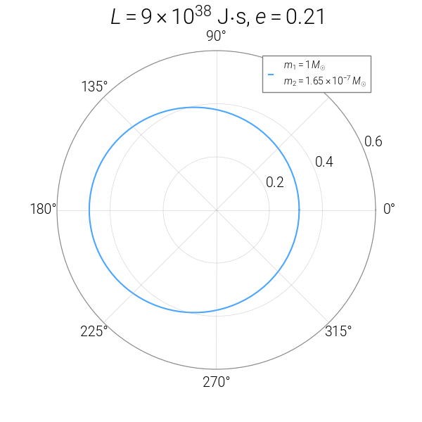
Step 7: plot the orbital track

We can now visualize the orbital track by plotting $(r(t), \varphi(t))$ in polar coordinates. Fortunately, Matplotlib makes it very easy to do this, with support for fine-tuning various features of the plot such as axis tick marks and color schemes.

# plot the equivalent-one-body orbital track
fig = plt.figure(figsize=(6, 6)) 
ax = fig.gca(projection='polar')  # use polar projection
ax.plot(phi, r/AU, '#4ba6ff',
        label='$m_1 = %s\,M_{\odot}$\n$m_2 = %s\,M_{\odot}$' % (
            _format_scientific(M1/MSUN), _format_scientific(M2/MSUN)))
ax.grid(True)

ax.legend(framealpha=1)
ax.set_rticks([0.2, 0.4, 0.6])
ax.set_title(r'$L=%s$ J$\cdot$s, $e=%.3g$' % (
    _format_scientific(L), ECC), va='bottom')
plt.show()

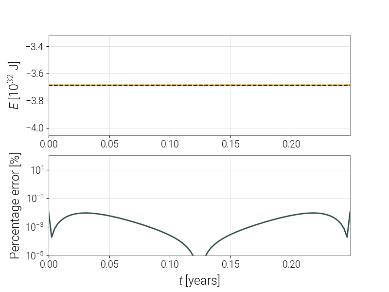
Step 8: check that energy is conserved

Huzzah, we have simulated Mercury's orbit! Now we'll want to do a couple of sanity checks to make sure our integration scheme did it accurately and faithfully. To examine this, recall that we already know the energy we expect the system to have is the constant E, a global variable. We can directly estimate the percentage error by numerically differentiating $r$, re-calculating the energy by hand for each data point using the condition

$$ E = \frac{1}{2} \,\mu \dot{r}^2 - \frac{GM\mu}{r} + \frac{L^2}{2\mu r^2}, $$

and then comparing these values to E.

Note: to take a derivative numerically, we will use the convenience function numpy.gradient. This is based on an algorithm that is second-order accurate everywhere except the first and last data points, where it is first-order accurate.

# check that the energy is conserved
rdot = numpy.gradient(r, dt)  # time derivative of r
energy = 0.5*MU*rdot**2 - G*M*MU/r + L**2/(2*MU*r**2)
error = numpy.abs((energy - E)/E)

# set up a figure
ty = t / 3.1536e7  # convert time to years
fig = plt.figure(figsize=(8, 6))

# plot the total energy
ax1 = fig.add_subplot(211)
ax1.plot(ty, energy/1e32, 'Orange', linewidth=2)
ax1.plot([ty[0], ty[-1]], [E/1e32, E/1e32], 'k--')
ax1.set_ylim([1.1*E/1e32, 0.9*E/1e32])
ax1.set_ylabel('$E$ [$10^{32}$ J]')

# plot the percentage error on a separate graph
ax2 = fig.add_subplot(212, sharex=ax1)
ax2.plot(ty, 100*error, 'DarkSlateGray', linewidth=2)
ax2.set_xlim([ty.min(), ty.max()])
ax2.set_xlabel('$t$ [years]')
ax2.set_ylim([1e-5, 100])
ax2.set_yscale('log')
ax2.set_ylabel(r'Percentage error [%]')
# show the figure
plt.show()

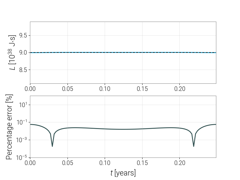
Step 9: check that angular momentum is conserved

Finally, we will do the same with the magnitude of orbital angular momentum, based on the condition that

$$ L = \mu r^2 \dot{\varphi}. $$

We will compare this to L, our global variable giving the expected angular momentum.

# check that the angular momentum is conserved
phidot = numpy.gradient(phi, dt)  # time derivative of phi
angmomentum = MU * r**2 * phidot
Lerror = numpy.abs((angmomentum - L)/L)

# set up a figure
fig = plt.figure(figsize=(8, 6))

# plot the orbital angular momentum
ax1 = fig.add_subplot(211)
ax1.plot(ty, angmomentum/1e38, 'DeepSkyBlue', linewidth=2)
ax1.plot([ty[0], ty[-1]], [L/1e38, L/1e38], 'k--')
ax1.set_ylim([0.9*L/1e38, 1.1*L/1e38])
ax1.set_ylabel('$L$ [$10^{38}$ J$\cdot$s]')

# plot the percentage error on a separate graph
ax2 = fig.add_subplot(212, sharex=ax1)
ax2.plot(ty, 100*Lerror, 'DarkSlateGray', linewidth=2)
ax2.set_xlim([ty.min(), ty.max()])
ax2.set_xlabel('$t$ [years]')
ax2.set_ylim([1e-5, 100])
ax2.set_yscale('log')
ax2.set_ylabel(r'Percentage error [%]')

# show the figure
plt.show()

Digging deeper

Now that we've simulated a complete orbit, consider the following:

Can you plot r and phi as a function of time? (Try to do it in the same figure but on separate graphs, like we did for the percentage error plots above.)
If you think of $r$ and $\varphi$ as oscillators, do they have the same frequency? (Remember: they should, because there can be no apsidal precession in the classical two-body problem.)
What does the motion look like when you transform back to the two-body model? Does it match what you expected?
What do the orbital features look like if you try to model different Solar System planets? How well are the energy and angular momentum conserved, numerically speaking?
Do you have to change anything about your initial conditions if you want to model parabolic or hyperbolic orbits? How well are the energy and angular momentum conserved, numerically?

Tides and the Roche potential

Simulating classical orbits using the RK4 method